In short
This tutorial aims to provide a comprehensive overview of best practices in storing and loading your dataset for training a deep learning model. For now, the focus is on saving and loading arrays/matrices/images data quickly and efficiently.
Why this tutorial:
To speed up your deep learning pipeline
To mitigate extensive and inefficient usage of the filesystem by saving each file separately, thereby affecting other users
- To provide a potential answer to: Disk quota exceeded
For who:
Any user saving and loading data (on Snellius) and requiring the data to be loaded quickly in their pipeline
How:
By following this tutorial
Finding the corresponding publicly available GitHub here
- Finding the prepared datasets (in this tutorial and more!) on Snellius at Available datasets and models on Snellius
Finding the right format to store your data and reading the data to train your model is a non-trivial task. The formatting choice of the data impacts the training speed and performance. Additionally, saving the data in a clever way encourages the filesystem to be healthy and efficient.
In the following sections, a variety of experiments will be carried out to provide pointers for the type of data and its usage. Also, some general tips will be given to further improve the data processing pipeline.
 TLDR (short answer):
for intuitive array-based data like images or matrices → HDF5
for larger datasets (>100GB) and images/matrices larger than 4KB each → LMDB
for general purpose and accessibility → uncompressed TAR/ZIP
for potential fast and willing to go down a rabbit hole → Petastorm
Table of Contents
The format for you
You have obtained your dataset either by collecting data yourself or retrieving a prepared dataset from a different source like the internet. Now the first step is to recognize the type of data you are dealing with. Start by asking this:
- What type are my samples? Do they represent images (.jpg/.jpeg/.png) or arrays/matrices? Is it saved in unordered tabular format consisting of numerical observations (.csv/.json/.txt)? Are we dealing with ordered time-series signals like audio or historical data (.csv/.json/.txt)?
- Do the samples contain corresponding ground-truth labels? Similarly, what type of data are the samples? Are all labels gathered in a single file, does each sample have its own label file or is the label saved together with the sample?
- How large (roughly) is the data? Is it possible to store locally (on /home/ for datasets smaller than 1GB) or on the project space/scratch space? Would the data fit in system memory all at once while training? (1 GPU node on Snellius has 450GB memory)
- How many individual files does the dataset contain? Is each sample stored separately? This question is especially relevant for the filesystem used to store the data. Having loads of of small files with each their own metadata degrades the performance of querying files and results in inefficient storage. In case of a large number of files, consider bucketing or packing the samples together. Below, we will list some examples.
Experiments
Filesystem All experiments are initially reported on the Snellius partitions. The majority of these partitions are mounted on a General Parallel File System (GPFS) which is a clustered file system commonly used by supercomputers. The parallel property of GPFS lies in having a storage that is divided by a fixed block size where the blocks are distributed across multiple disks, allowing the reading operations to be performed in parallel.
Framework The framework was set up in Python and employs PyTorch as the dataloader manager.
Datasets Three different image datasets are employed with different file sizes as well as image/array dimensions (these datasets can be found prepared and processed on Snellius at Available datasets and models on Snellius)
- CIFAR10: an image classification datasets consisting of 60,000 32x32x3 color images
- ImageNet10k: a random subset of 10,000 images from the original ImageNet10k image database. The images are of different resolutions and include both grayscale and color images.
- FFHQ: a high-resolution dataset of human faces with 70,000 color images of 1024x1024x3.
Arrays/Matrices/Images
 General tips:
Binary data
While deciding on what type of data format to use, it is recommended to use a format which uses serialization such that the data is saved in binary format. One advantage of converting the data into bytestreams is to reduce the disk space. More importantly, bytes are generalized data types and can easily be interpreted across other platforms, operating systems and programming languages. For example, both an NxD array as well as a string or number can be described in bytes. Luckily, most packed data formats already have or explicitly require the data to be transformed into binary data, thus you do not need to worry about implementing yourself or needing a certain skill set for this.
![]() Take away: to save disk space and enable easy access across machines, choose a packed data format which implicitly serialize the data or convert the data into a binary format yourself (instead of storing the data in raw format like csv/txt/json or arrays).
Take away: to save disk space and enable easy access across machines, choose a packed data format which implicitly serialize the data or convert the data into a binary format yourself (instead of storing the data in raw format like csv/txt/json or arrays).
Compression/Encoding
Many packed data formats do not save the data compactly as to minimize the disk space. Rather, the aim for these formats is to optimize read and write performance. In the case where the size your data is of high importance, for example, having a large dataset with only limited storage space, it may be worthwhile to store the data with compression. These compression methods can be employed as a tool to reduce the used disk size by encoding the data during writing and decoding upon accessing and reading. For packed data formats, we can utilize compression on two levels: on sample level and on archive level. We further divide compression and encoding as follows: compression is a general method to effectively reduce the size of your data by applying compression algorithms. Some algorithms will reduce the quality and reconstructing the original data back from the compressed data results in a loss of information. Other algorithms are able to perform lossless compression such that the full information of your data is compressed. The more information you allow the algorithm to lose, the lower the size of your compressed data will be. With encoding we refer to a specific type of compression. One such an example includes encoding your images with specific information about imagery data such that the compression method is more informed to a more effective technique of compression.
Sample-level compression/encoding Applying compression per sample entails encoding the individual data parts directly and storing the compressed result to the disk. For images, instead of saving a NxMx3 array of intensity values, one can employ an image compression method and save the compressed data instead. In a traditional deep learning setting where we prefer not to lose any important information, lossless compression is favored such as PNG or WEBP. As the majority of the data formats only handle with binary data, the samples also need to be serialized into a stream of bytes. Combining compression and serialization by first encoding the raw data and storing the compressed data, the disk space is further minimized as compared to saving the serialized data. The trade-off here is the extra computational overhead introduced by the encoding and decoding of the compression method for the writing and reading speed.
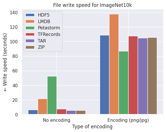
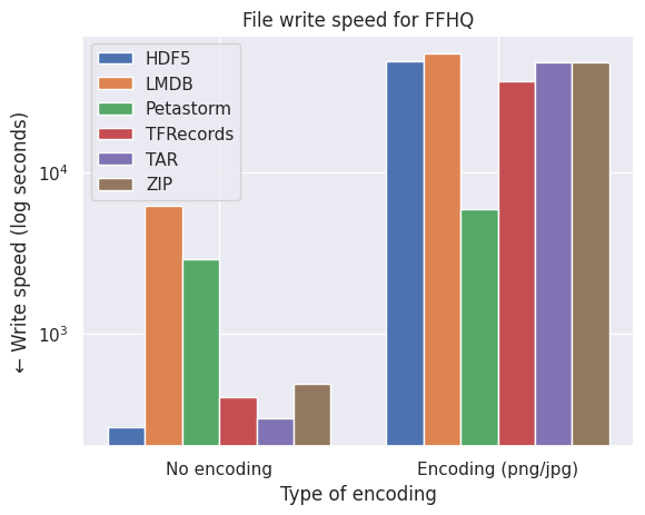
Below are graphs of the effect of disk space on three different image datasets. No compression implies directly encoding the pixel arrays from NumPy uint8 format into a stream of bytes while encoding refers to PNG (CIFAR10 and FFHQ) or JPEG (ImageNet10k) compression.
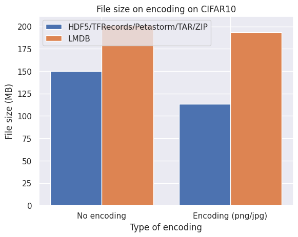
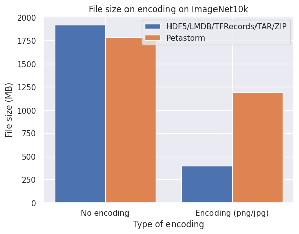
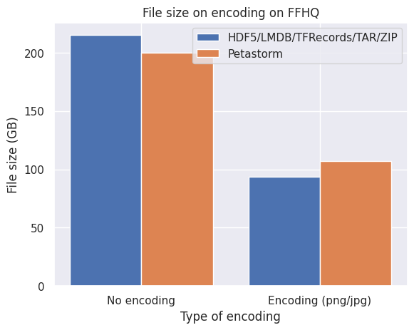
What we observe from the bar plots above:
- Encoding the images individually does effectively reduce the required disk space.
- LMDB is inefficient for datasets with small files around the block size or smaller of your filesystem (4kB and smaller) which is the case with CIFAR10.
- Petastorm is less flexible in encoding the images and is not always able to retain the quality and level of compression of the original images.
- HDF5/TFRecords/TAR/ZIP are efficient and consistent for different datasets and settings.
Not so quick! Encoding and compressing takes time. While we generally only want to convert or pack our data once, it can be worthwhile to see the effect of the speed of writing the encoding vs. unencoded data to the format. See the graphs below.
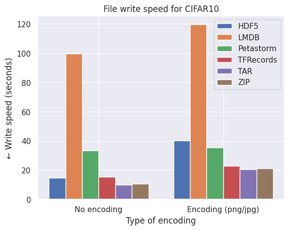
What conclusions do we draw from the bar plots above:
- LMDB is also inefficient in terms of speed due to the smaller files of CIFAR10 which are around the size of the block size (4kB).
- LMDB (at least my implementation) is not efficient in writing individual files in a multiprocess settings. The write transactions are expensive and one can significantly improve the LMDB write speed by writing batches of images to the file.
- Petastorm becomes progressively faster on encoding on larger datasets (note the log scale of FFHQ) but at the cost of required disk space and freedom of settings different compression methods, as observed by the graphs on file size above.
- HDF5/TFRecords/TAR/ZIP are efficient and consistent for different datasets and settings.
Cool but what about read speed? Converting your data to the right format is usually done only once if work with a static dataset (does not need to be updated regularly), so these preprocessing steps are less important than loading the data for our model. Often in our pipeline we want to access the same file and same array/image multiple times (number of epochs) so efficiently getting the data from the format to our code is crucial. To see the results, please refer here.
![]() Take away: if disk space is important or you have a high number of workers available (>64), encoding the data, for example with image encoding, can effectively reduce the disk footprint while not affecting the read performance too much. If the speed of loading the data is major decision factor then directly serialize and save the data with formats like HDF5/TAR/ZIP.
Take away: if disk space is important or you have a high number of workers available (>64), encoding the data, for example with image encoding, can effectively reduce the disk footprint while not affecting the read performance too much. If the speed of loading the data is major decision factor then directly serialize and save the data with formats like HDF5/TAR/ZIP.
Archive-level compression Besides compressing or encoding the files individually, we can also perform compression on the entire packed file or archive. While applying compression on this level results in an even lower required disk size, one should be aware of the consequences. In data formats such as HDF5 or ZIP compression can easily be enabled. However, most compression methods are not parallelizable (like .tar.gz.) which may result in a very slow writing and especially reading performance. Only in a setting with careful consideration where the packed data files are thoughtfully divided into multiple files where each workers can apply compression individually on the file may it be worth to use compression on archive-level.
![]() Take away: compressing the archived file itself may be useful to transfer data to other platforms, but can noticeably impact the i/o performance of your data, so only use if disk space availability is scarce.
Take away: compressing the archived file itself may be useful to transfer data to other platforms, but can noticeably impact the i/o performance of your data, so only use if disk space availability is scarce.
Cache
In the context of dat aloading, caching entails saving (a part) of your data to a temporary fast disk space which will hold the data separately instead of reading the file multiple times. Of course, we are restricted to how large this temporary disk space is. Smaller datasets like CIFAR10 (<1GB) usually fit in the cache memory and storing the data in the cache will avoid repeatedly loading the data from disk and drastically increase the data loading pipeline. In simple terms, you can cache by opening all files and reading the content, say images, and appending them in a list or array such that they are quickly accessible by the system. For PyTorch, this would happen in the __init__ of the dataset instance. However, for larger dataset this may not be feasible so we are resorted to partial caching where we each time only store part of the data, or no caching at all. The codebase as of now only supports no caching as this works in every setting independent on dataset type or size. However, using (partial) caching in a methodical way will improve the speed of overall pipeline.
Image reading
For loading images of PNG or JPEG extensions from disk or an archived file, it can be useful to check the library used to read the images. A common and powerful library is Python Imaging Library (PIL). The image library supports multiple file formats, basic image processing techniques and fast access to the data. On top of that, the PyTorch torchvision transformations work directly on PIL image instances without requiring any type conversion. While already PIL is a good start for general purpose image loading, extension-specific optimizations are implemented by external libraries for a faster reading time. For PNG such an alternative is pyspng which is a small package to efficiently load images directly in NumPy arrays. For JPEG images, PyTurboJPEG is a Python wrapper of turbojpeg for fast encoding and decoding of JPEG extensions.
Below are two experiments on a PNG and JPEG dataset and alternatives to PIL for reading images with specific extensions.
| CIFAR10 | Time elapsed for 1 epoch (in seconds) |
|---|---|
| PIL | 15.5 |
| pyspng | 9.7 |
| ImageNet10k | Time elapsed for 1 epoch (in seconds) |
|---|---|
| PIL | 44.1 |
| PyTurboJPEG | 38.3 |
![]() Take away: when loading images saved as image extensions (in packed data formats like ZIP and TAR or for smaller datasets directly on disk), consider using external libraries (pyspng for PNG, PyTurboJPEG for JPEG) for an improved read time.
Take away: when loading images saved as image extensions (in packed data formats like ZIP and TAR or for smaller datasets directly on disk), consider using external libraries (pyspng for PNG, PyTurboJPEG for JPEG) for an improved read time.
- Image file extension (PNG vs JPG/JPEG vs TIFF)
One big difference between these formats is the way the images are compressed. In JPG/JPEG, the pixels are saved with a lossy compression method. As a result, JPEG files usually are lower in size and do not capture the original quality, but rather a percentage of the original quality, usually around 95%. In contrast, PNG employs a lossless compression method where the original pixel values are retained but at the cost of a higher image file size. For a human, the difference between JPEG and PNG is hard to see by eye. Of course since the actual pixel values between these formats are different the computer is able to differentiate between a JPEG and PNG image. In the end, the image array is taken as input to the neural network and therefore the choice of file extension affects the performance of the network. Since JPEG are smaller, they may speed up training while PNG is able to maintain the best picture quality. Keep in mind that for inference the pre-trained model on PNG images may perform inference well on new JPEG images but this not hold vice versa.
![]() Take away: Generally, the original image format the data comes in works fine. Matching the inference image extension with the extension in the training dataset is of high importance. Only in case for larger networks or specific scenario may it be worth to train the model on JPEGs and potentially finetune on PNG images.
Take away: Generally, the original image format the data comes in works fine. Matching the inference image extension with the extension in the training dataset is of high importance. Only in case for larger networks or specific scenario may it be worth to train the model on JPEGs and potentially finetune on PNG images.
 Packed Data Formats
Disk (PNG/JPG/JPEG/TIFF)
When downloading a dataset from an online source, the data samples are generally compressed into a single file for a faster download and transfer to the filesystem. After extracting the file on the system, the data samples often have a one-to-one relation with the sample, that is each sample is saved separately as an image. Individually opening the files during training may be slow as each image and its metadata needs to be read. Also, the filesystem experiences inefficiency as the size of the saved images may be lower than the block size of the filesystem, leading to images being saved with unused empty space within the block while also reserving many inodes. Instead, it would be more ideal to collect a set of samples and group them together into a single file.
Pros ![]()
- Files are easily accessible for manual inspection of the data at any time
- No extra coding is required to convert the data
Cons ![]()
- A large number of individual files may degrade the performance of the filesystem, especially in the case of Snellius with its shared parallel filesystem
- Loading each data sample directly from disk is slow
- Requires a high number of workers
![]() Take away: only use individual images in case for very small datasets (< 1GB) or a limited number of images (< 1.000 samples). While it is more user-friendly, the filesystem and your data pipeline will be affected and we highly recommended using a different format
Take away: only use individual images in case for very small datasets (< 1GB) or a limited number of images (< 1.000 samples). While it is more user-friendly, the filesystem and your data pipeline will be affected and we highly recommended using a different format
ZIP/TAR
One way to alleviate the exploding number of files being stored is to pack the samples into a single file, or group the files in a number of shards. This way, the finite and sometimes scarce number of inodes is heavily reduced and chunking the saved files is better optimized (which is better for the filesystem and thus your speed!). During training the file handler of the packed file can be cached to quickly retrieve the samples from the grouped file.
A common compression method is the ZIP format. Each file is first compressed individually and then added to the archive to allow for random access. This allows for fast extraction of individual files without sequentially going through the archive or unpacking. The type of compression is crucial as it determines the quality of the samples. In addition, decompressing each file again during training introduces overhead. In general, the compression level is zero, meaning the samples are compressed lossless (also called deflated) and the original quality is preserved. In practice, the images are serialized into a stream of bytes which represent the original image and the byte stream is archived. Upon unpacking, the byte streams are deserialized and converted back to images.
As files of different types can be archived together, the metadata file with the labels in JSON format is compressed in the same zip file.
TAR is also a common packed data format which compresses the entire output file instead of separate files like ZIP.
Pros ![]()
- Manually inspecting the data is still intuitive for smaller packed files
- General format to share across platforms and internet
- Sometimes data already comes in ZIP so does not conversion to other format
Cons ![]()
- Not optimized for fast reading
- Decompressing takes a lot of time for TAR files due to unparallelizable decompression methods (but can be cached)
![]() Take away: ZIP/TAR is a good alternative to combine speed while also still be able to checkout the data manually. It does need a few tricks in the code for parallel reading but this is implemented in the GitHub
Take away: ZIP/TAR is a good alternative to combine speed while also still be able to checkout the data manually. It does need a few tricks in the code for parallel reading but this is implemented in the GitHub
HDF5
Hierarchical Data Format (HDF5) is a hierarchical database contained and described in a single file (.h5 or .hdf5). While HDF5 is popular among GIS systems due to linking various types of properties to a specific sample in a structural manner, the format can also be employed in other scenarios. A HDF5 file supports large heterogeneous data which means that tabular data as well as metadata can be stored while also enabling the storage of variable high dimensional data such as images, all within a single hierarchical data file. The data types are mostly handled with NumPy which allows for a direct and straightforward implementation for array-based data.
Pros ![]()
- All samples are compressed into a single file for less disk space
- Built-in NumPy functionalities
- Features a hierarchy for saving structural data
Cons ![]()
- Within the hierarchy, the arrays need to have identical shapes
- Not intuitive/optimized for non-numerical data (labels)
![]() Take away: for a straightforward datasets of arrays/images, HDF5 works reliably and consistenly. It shines even more in structured arrays, but does need setting specific array details (like a fixed shape). For ImageNet, we had to resize all images to identical shape to use HDF5.
Take away: for a straightforward datasets of arrays/images, HDF5 works reliably and consistenly. It shines even more in structured arrays, but does need setting specific array details (like a fixed shape). For ImageNet, we had to resize all images to identical shape to use HDF5.
LMDB
Lightning Memory-Mapped Database Manager (LMDB) is a database management library built on B+ trees. LMDB was optimized for efficient read transactions and allows for multiple threads in multiple processes for reading. The database library is composed of memory-mapped files with key-value pairs where keys are uniquely identifiable IDs. For images, the key can be the file name or an integer index. The values expects bytes and thus for images serialized image arrays in a grouped Python object such as a tuple or a list together with its corresponding serialized label.
Pros ![]()
- Optimized for fast read transactions
Cons ![]()
- Introduces overhead if the arrays or images are smaller than the block size (<4KB files)
![]() Take away: LMDB is indeed lightning fast for read, although saving the data in this format may be more time-consuming compared to the others.
Take away: LMDB is indeed lightning fast for read, although saving the data in this format may be more time-consuming compared to the others.
Petastorm/Parquet
Petastorm is a library developed by Uber that leverages fast access and storage in Apache Parquet format. Traditionally, ordered columnar formats commonly found in databases are unable to store multidimensional data such as images. By extending the .parquet data files with petastorm's Unischemas, multidimensional tensors can be directly stored in the format. In addition, the unischema supports transferring the structure directly to the native PyTorch and TensorFlow readers. Petastorm uses a PySpark environment to efficiently manage distributed data processing.
Pros ![]()
- Scales well with number of workers
- More advanced reader options like selective reading, local and global shuffling and column splitting
- Huge potential if you know what you are doing
Cons ![]()
- Huge potential if you know what you are doing
- Extra software (Java for PySpark) needed
- Too many settings to tune for a really streamlined process
- Requires arrays to be a fixed and identical shape
![]() Take away: while Petastorm is 'smarter' compared to the others by having more functionalities and implicit caching, this often results in unoptimized reading and writing operations. Only consider Petastorm if you are confident with HPC and your data.
Take away: while Petastorm is 'smarter' compared to the others by having more functionalities and implicit caching, this often results in unoptimized reading and writing operations. Only consider Petastorm if you are confident with HPC and your data.
TFRecords
Tensorflow developed their own binary data format to process dataset seamlessy with the library and named it TFRecord. To store data in a TFRecord file, the sampes and labels are converted to a byte string according to a pre-defined schema and efficiently serialized by a protocol buffer. During the data loading process, the buffer will be streamed in segments for fast access and supports the Tensorflow processing tools such as shuffling, batching etc.
Note, since TFRecords is designed and optimized for Tensorflow, converting the dataset to a PyTorch (iterable) dataloader may result in reaching suboptimal performance.
Pros ![]()
- Extensive support for Tensorflow
Cons ![]()
- Only natively compatible with Tensorflow and requires additional code to run on PyTorch
- Limited flexibility
![]() Take away: TFRecords might shine more in Tensorflow, but already this is an issue as it cannot be directly used in other frameworks like PyTorch without custom software. From our experience, having your data in a more generalized format is the way to go.
Take away: TFRecords might shine more in Tensorflow, but already this is an issue as it cannot be directly used in other frameworks like PyTorch without custom software. From our experience, having your data in a more generalized format is the way to go.
 So which is the fastest
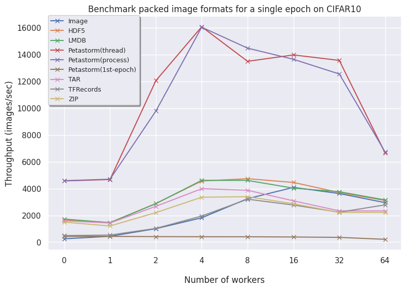
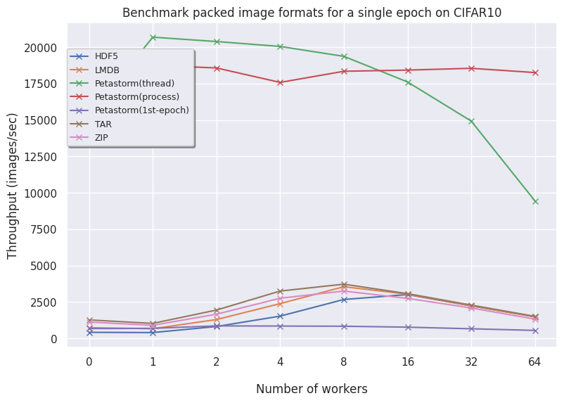
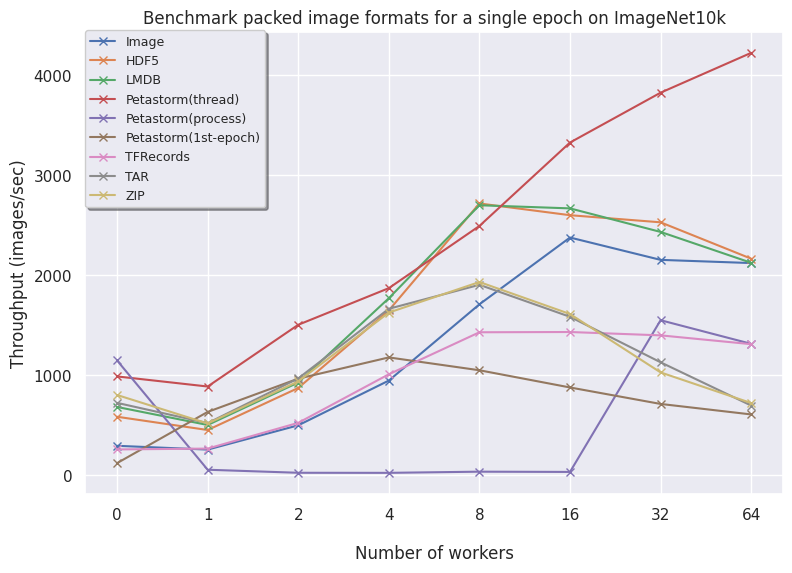
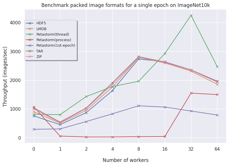
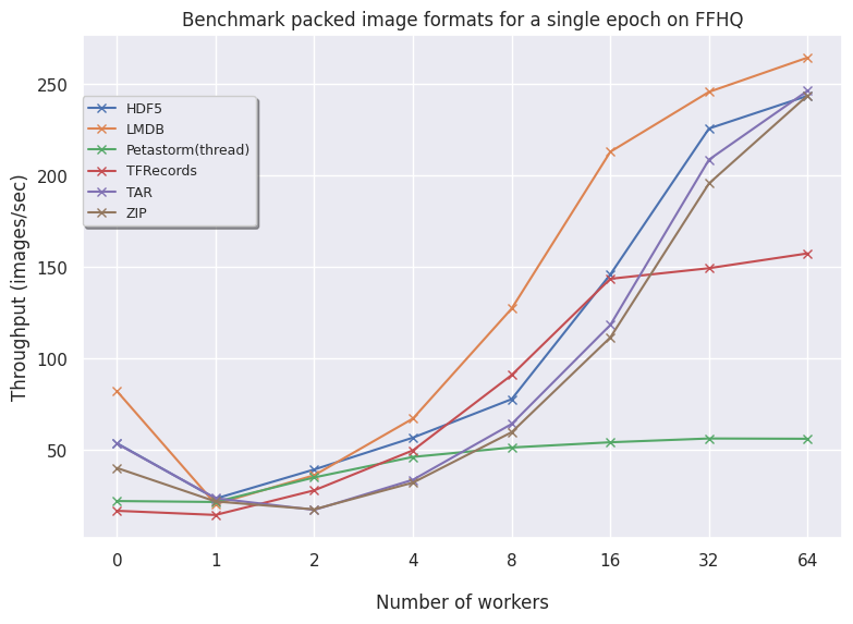
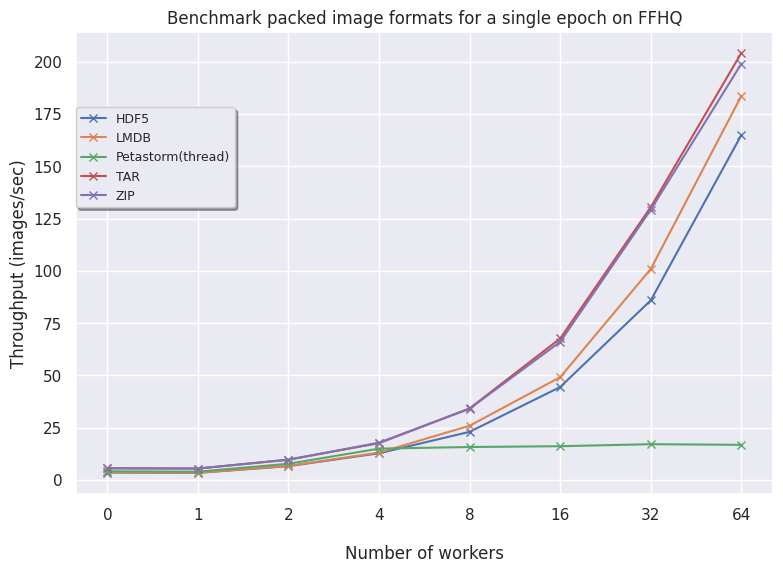
Below are plots for the CIFAR10, ImageNet10k and the FFHQ image datasets. The results are reported with a fixed batch size of 16 and we allow the dataloaders to have a warm start (only the second epoch is timed).
On the left, the uncompressed data is shown. On the right, the encoded plots are visualized.
CIFAR10:
ImageNet10k (subset of ImageNet):
FFHQ:
Let's investigate our findings per data format:
- Image contains individual files saved on disk and needs a high number of workers to compare to the other formats. For larger datasets, the files are too big and inefficient to store on the filesystem so these are omitted. In conclusion, using individual files only is advised with a very small dataset or low number of files.
- HDF5 is consistently fast across all dataset and is a very good option for array-based data.
- LMDB for larger datasets (FFHQ) is favorable as higher volumes of data benefit from having an optimized read procedure as LMDB employs. For smaller data, LMDB is not efficient in saving data so other alternatives like HDF5/TAR/ZIP are preferred.
- Petastorm has functionalities to use either a multithreaded or multiprocessing dataloader. On CIFAR10, we notice Petastorm is really fast but this might be due to implicit caching happening in the backend (saving the entire CIFAR10 dataset in cache as it is relatively small). Preparing this caching costs extra time as observed from the timings of the 1st (first) epoch. For larger datasets like FFHQ and already ImageNet subset it is not possible to cache the entire dataset and in this case Petastorm does not set superior timings, also due to the highly adjustable parameters.
- TFRecords perhaps does not shine in a PyTorch setting as we see from the graphs in all datasets but inherently this does pose a problem as TFRecords is not a general format and needs additional modules. TFRecords is omitted for the encoding benchmarks as the protocol buffer does easily allow for opening image encodings. In terms of speed, it is outperformed by other alternatives.
- TAR is consistent but does not scale well to larger TAR files without caching the names of the files. This is because getting the names (
getmembers()) is a very time-consuming operation. By caching the members in a separate file, this expensive operation is avoided and TAR is very similar to ZIP. - ZIP is also consistent and scales well. In the case of encoding your images, then TAR and ZIP naturally scale well. In general, having your data zipped is a good approach both for transferring data as well as loading data.
Other conclusions:
- For larger datasets, more workers is better!
- Default number of workers of PyTorch dataloader is 0, so setting this parameter
num_workers=8already highly improves the data loading pipeline - While encoding the images does decrease the disk load, the read speed is impacted up to a factor of 5x (on FFHQ with
num_workers=8)
Tags:
data, data format, dataset, dataloader, data loading, packed, compressed, jpg, jpeg, png, image, pytorch, tensorflow, extension, snellius, lisa